Design
Finite element analysis.
Time and setting
This research was conducted on September 2, 2018 at Digital Medical Center of Inner Mongolia Medical University.
Subjects
One patient (male, 12 years, 52 kg) with non-skull base atlantoaxial disease who underwent imaging in the Second Affiliated Hospital of Inner Mongolia Medical University in February 2016 was enrolled in this study. Diagnosis was confirmed by three senior doctors of orthopedics and imaging with a title of associate chief physician or higher. No dyskinesia or abnormal imaging findings were observed. The patient’s family members signed the informed consent.
Materials
A 64-slice spiral CT scanner was provided by General Electric, USA. Materialise's Interactive Medical Image Control System 16.0 software (Materialise, Belgium), 3 matic8.0 software (Materialise, Belgium). The material parameters of steel plate and screw are shown in the Table 1.
.jpg)
Methods
CT scanning
All CT data were obtained by a 64-slice spiral CT scanner. The following scan parameters were used: slice thickness 0.625 mm, pitch 0.921, slice gap 0.5 mm, current 250 mA, voltage 120 kv, bone window, and 150 scanned slices.
Three-dimensional reconstruction
Experimental work was completed in the Department of Computer Technology Teaching and Research, College of Computer Information, Inner Mongolia Medical University. Eligible CT data were stored in DICOM format in a mobile hard disk. Mimics 16.01 software was open, and the Import Image button in FILE sequence was clicked to import DICOM files. Before importing, four directions, including anterior, posterior, left, and right, were selected through three cross sectional images. After the directions were confirmed, the Convert button below was clicked to enter the formal image operation interface. Four operation boxes (left to right, top to bottom) were coronal, horizontal, sagittal, and three-dimensional interfaces, respectively (Figure 1). The shortcut key Thresholding was selected to set the gray value of bone scintigraphy. The gray value was between 226 and 3071 HU[9]. The Region Growing button was clicked to apply a green mask to the bone in the image. A green mask was applied to all areas within the gray-value range in all images by the software (Figure 2). Next, the Edit Masks button was clicked to manually modify the bone tissue boundaries in each slice by comparing to the three different sections, to wipe soft tissue images with a high gray value, and to fill mask cavities caused by cancellous bone. Then, calculated three-dimension was selected to superpose and reconstruct the plane mask. After reconstruction, the Smoothing button in the Tool sequence was clicked to obtain clear images of the atlantoaxial joint (Figure 1).
.jpg)
Reconstruction, introduction, registration and assignment of the transoral anterior atlantoaxial plate
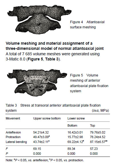
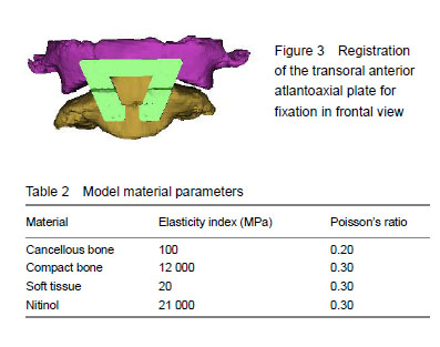
The transoral anterior atlantoaxial plate was designed with the reference to diameters of the patient using the Pro/ENGINEER 4.0 (Parametric technology corporation, USA). The plate and screws are shown in Figure 2. The following parameters were measured: distance between right and left upper screw hole centers, 26 mm; distance between right and left lower screw hole centers, 8 mm; plate height, 13 mm; distance between upper and lower screw hole centers, 12 mm; screw diameter, 2.5 mm; screw length, 14 mm. The reconstructed three-dimensional model of the plate and screws was introduced into Mimics 16.01 (Materialise, Belgium) and registered according to the requirements of a typical transoral anterior approach, followed by surface and volume mesh generation and material assignment[10] (Figure 3, Table 2).
Stress loading
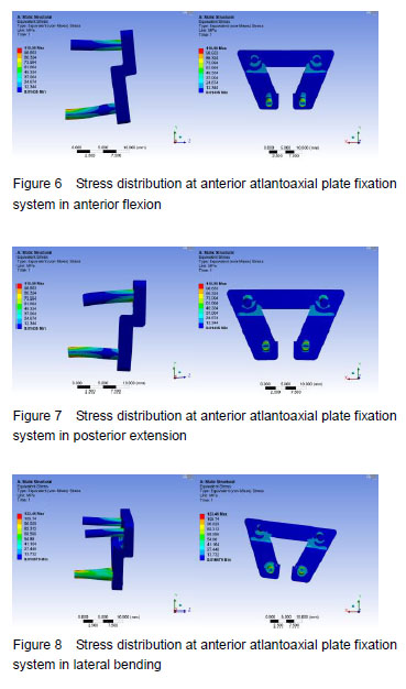
According to the head to body weight ratio[11], a 60-N load was applied vertically at the left and right lateral masses of the atlas, and evenly distributed at each node on the atlas surface. In addition to the vertical load, a 15-N • m moment was applied at the left and right lateral masses of the atlas. The lower surface of the axis was fixed. Anterior flexion, posterior extension, and lateral bending were simulated. The results were expressed in qualitative and quantitative terms. In qualitative terms, a stress distribution cloud diagram was used, with different colors representing different forces. In quantitative terms, stress was measured at 10 uniformly distributed points in the area of stress concentration of the target object.
Main outcome measures
Stresses of upper/lower screw bottom were measured.
Statistical analysis
Data are expressed as mean ± standard deviation, and analyzed using SPSS 13.0 (SPSS, Chicago, IL, USA). The stress at the same point between the three movements was compared by analysis of variance. The stress at the same point in the same movement between the upper and lower screws was compared using a paired t-test. P < 0.05 was considered statistically significant.